Stateful Graph Algorithms in Haskell
- Motivation
- Introduction
- How to Run
- Implementation Details
- Code Reference
- Testing
- Referenced Paper
- Appendix
Motivation
In my Programming Languages course as part of my graduate program (CS 421 at UIUC by Professor Beckman in Summer ‘23), I was got extensive experience using Haskell, a functional programming language. This type of language is much different than object-oriented languages like Python and C++, of which I was much more familiar.
There’s a lot more I could and should say about differentiating Haskell from these object-oriented languages, but here are a few highlights:
- the languages is built entirely around functions, not variables or classes (per se).
- there are NO
fororwhileloops; only recursion. - a properly defined function reads surprisingly like mathematics, which is like music to my ears after majoring in math as an undergrad.
Given these big differences with Haskell, an important aspect of the language revolves around the idea of managing state. As a final project for the course, I decided to investigate this concept further with respect to graph algorithms, and what follows here is a slightly modified version of my final project report.
Introduction
I have a special interest in graph algorithms, and I was impressed with the elegance and simplicity of binary search tree implementation using the Haskell programming language as demonstrated in class by Professor Beckman (see Appendix). While trees are acyclic, graphs in general can contain cycles. In such cases, as pointed out in the King & Launchbury paper linked below, while performing a depth-first search of a graph there is a need to maintain state in the form of the knowing which nodes have already been visited. Conveniently, as the authors also describe, we can “use monads to provide updatable state,” and we can apply this idea to maintaining a set of visited nodes.
Nevertheless, I have found the logic of the Monad type class to be difficult to grasp but its utility is undeniable. With this in mind, my goal for the final project was to combine these two concepts of graph algorithms and managing state, with the hopes of furthering my understanding of both.
Therefore, I implemented the following in Haskell, as per my project proposal:
- A
Graphdata type that allows for cycles (i.e., not just for trees). - A
traversalfunction that returns an in-order traversal of a graph via depth-first search. - A
shortestPathLensfunction that returns the number of hops in the shortest path between two nodes of a graph via breadth-first search. - The above two functions make use of monads to maintain state.
Furthermore, I implemented several additional features that seemed warranted:
- For the purpose of comparing with the monadic implementations of the two functions above, I also implemented them by simply passing state variables as arguments.
- I created a small Python module for the purposes of testing my Haskell implementations, relying heavily on the
networkxlibrary. More details in the Testing section below. - I created a REPL of my Haskell application to allow the user to more easily test and play with the algorithms for whatever graphs the user might please, either by reading a pre-built graph from a text file or by manually entering graph edges to create a custom graph.
In the end, I was surprised to learn that manually passing state variables resulted in more concise code compared to the monadic implementations. To be sure, using a state monad allowed for functions with fewer parameters, but repeatedly accessing and modifying the state resulted in more lines.
How to Run
- download the code (e.g.,
git clone https://github.com/dougissi/stateful-graph-algos-haskell.git) - navigate to the project directory (e.g.,
cd stateful-graph-algos-haskell) - run all unit tests via
stack test - enter REPL via
stack run
Implementation Details
Graph data type
To test my understanding, I developed my own Graph data type as opposed to using the Data.Graph module or copying the implementation found in the referenced paper. While my implementation may lack some of the robustness of these other implementations, it makes up for it in is clarity and simplicity.
Nodes are represented as integers. A graph is simply a mapping between a node and its neighbors.
import Data.Map as M

type Node = Int
type Neighbors = [Node]
type Graph = M.Map Node Neighbors
Building a Graph
For my purposes, I defaulted to creating undirected graphs.
A graph can be built by passing in its list of edges. For example, consider the following graph of a triangle.
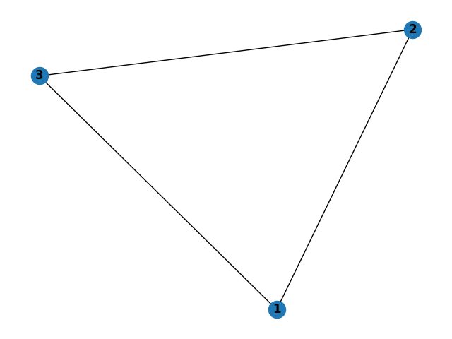
It can be built from the REPL by simply entering the information on the three edges:
> graph (1,2) (1,3) (2,3)
Graph: 1->[2,3] 2->[1,3] 3->[1,2]
The order of nodes within an edge is irrelevant. Entering (1,2) as an edge is equivalent to entering (2,1).
The order of edges matters only insofar as the neighbors of a given node are added in order of appearance. For example, if I enter graph (1,3) (1,2), then node 1’s neighbors will be ordered [3,2] (likewise the neighbors of nodes 2 and 3 with both be [1]).
You can replace the currently loaded graph by simply entering a new graph.
The underlying implementation of building a graph can be found here.
In-Order Traversal
To maintain the state of an in-order traversal of a graph g starting at src, we ought to keep track of two items:
- which nodes have been visited (
vin code below) - the current state of the traversal (
tin code below)
type VisitedNodes = S.Set Node
type Traversal = [Node]
type TraversalState = (VisitedNodes, Traversal)

traversalM :: Graph -> Node -> State TraversalState Traversal
traversalM g = dfs
    where
        dfs root = do
            (v, t) <- get
            case M.lookup root g of
                Nothing        -> return t
                Just neighbors -> do
                    let v' = S.insert root v  -- mark root as visited
                        t' = t ++ [root]  -- add root to traversal
                    put (v', t')
                    loop neighbors  -- do dfs on nonvisited neighbors

        loop [] = do (_, t) <- get  -- no remaining neighbors
                     return t

        loop (i:is) = do (v, _) <- get
                         if i `S.notMember` v
                            then do _ <- dfs i  -- continue traversal
                                    loop is
                            else loop is        -- try next neighbor
For the purpose of comparison, here is a non-monadic implementation
type Traversal = [Node]

traversal :: Graph -> Node -> Traversal
traversal g src =
    let (_, t) = dfs src S.empty []
    in t
    where
        dfs root v t =
            case M.lookup root g of
                Nothing -> (v, t)
                Just nbrs ->
                    let v' = S.insert root v  -- mark root as visited
                        t' = t ++ [root]  -- add root to traversal
                    in loop nbrs v' t'  -- do dfs on nonvisited neighbors
        loop [] v t = (v, t)  -- no neighbors remaining
        loop (i:is) v t =
            if i `S.notMember` v
                then let (v', t') = dfs i v t  -- continue traversal
                     in loop is v' t'
                else loop is v t  -- try next neighbor
From the REPL, once the user has built a graph, a traversal from a given node can be obtained.
> graph (1,2) (1,3) (2,3)
Graph: 1->[2,3] 2->[1,3] 3->[1,2]
> traversal 1
[1,2,3]
Shortest Path Lengths
Central to being able to calculate shortest path lengths between nodes is to be able to perform a breadth-first search. Now, in order to maintain state of a graph g when performing a breadth-first search between start node s and end node e, we ought to keep track of
- which nodes have been visited (
vin code below) - a queue of which nodes to check next, each linked with its depth from starting node (
qin code below)
type VisitedNodes = S.Set Node
type Depth = Int
type Queue = [(Node, Depth)]
type StateBFS = (VisitedNodes, Queue)

bfsM :: Graph -> Node -> Node -> State StateBFS Int
bfsM g s e = do
    case M.lookup s g of
        Nothing -> return (-1)          -- start not in graph
        Just _  ->
            case M.lookup e g of
                Nothing -> return (-1)  -- end not in graph
                _       -> do           -- start, end both in graph
                    (v, q) <- get
                    put (v, q ++ [(s, 0)])  -- add start to queue
                    aux                     -- process queue
    where
        aux = do
            (v, q) <- get
            case q of
                []           -> return (-1)   -- queue empty; fail
                ((i, d): q') -> do            -- "pop" next node
                    if i == e                 -- win; return depth
                        then return d
                    else if i `S.member` v    -- already visited; skip
                        then do put (v, q')
                                aux
                    else do
                        case M.lookup i g of  -- get node's neighbors
                            Nothing   -> do put (v, q')  -- none; skip
                                            aux
                            Just nbrs -> do   -- add neighbors to queue
                                let q'' = q' ++ [(x, d + 1) | x <- nbrs]
                                    v' = S.insert i v
                                put (v', q'')
                                aux
For the purpose of comparison, here is a non-monadic implementation
type Depth = Int

bfs :: Graph -> Node -> Node -> Depth
bfs g s e =
    case M.lookup s g of
        Nothing -> -1              -- start not in graph
        Just _  ->
            case M.lookup e g of
                Nothing -> -1      -- end not in graph
                _       ->         -- start, end both in graph
                    let v = S.empty   -- initialize empty visited set
                        q = [(s, 0)]  -- initialize queue with start
                    in aux v q        -- process queue
    where
        aux _ []           = -1        -- queue empty; fail
        aux v ((i, d): q')             -- "pop" next node
            | i == e       = d         -- win; return depth
            | S.member i v = aux v q'  -- already visited; skip
            | otherwise    =
                case M.lookup i g of   -- get node's neighbors
                    Nothing -> aux v q'  -- none; skip
                    Just nbrs ->         -- add neighbors to queue
                        let q'' = q' ++ [(x, d + 1) | x <- nbrs]
                            v' = S.insert i v
                        in aux v' q''
There is little work to be done once we have a working breadth-first search algorithm to extend it to find the shortest paths between all nodes (if a path exists, of course). See here for the implementation.
From the REPL, once the user has built a graph, the list of shortest paths can be obtained.
> graph (1,2) (1,3) (2,3)
Graph: 1->[2,3] 2->[1,3] 3->[1,2]
> shortestPathLens
[(1,[(2,1),(3,1)]),(2,[(1,1),(3,1)]),(3,[(1,1),(2,1)])]
The three items of the output array of shortestPathLens can be interpreted as:
- For node
1, the shortest path to node2is 1, and the shortest path to3is 1 - For node
2, the shortest path to node1is 1, and the shortest path to3is 1 - For node
3, the shortest path to node1is 1, and the shortest path to2is 1
Code Reference
All the code for this project can be found at github.com/dougissi/stateful-graph-algos-haskell.
Here is a reference for the various components.
- stateful-graph-algos-haskell/
- app/
- Main.hs — REPL
- graphs/
- python/
- graph_algos_networkx.py — Python submodule using
networkxto check test cases and visualize graphs
- graph_algos_networkx.py — Python submodule using
- src/
- GraphAlgos.hs — non-monadic implementations of graph algos
- GraphAlgosMonad.hs — monadic implementations of graph algos
- GraphsCommon.hs — graph construction and common functions
- Parse.hs — parsing graph edges entered into REPL
- test/
- Spec.hs — HUnit unit tests
- README.md
- app/
Testing
Overview
A series of unit tests were created using the HUnit library to confirm the accuracy many aspects of the codebase, particularly that of the traversal and shortest path length algorithms. The complete test code can be found at ./test/Spec.hs.
Even for simple graphs, it can be difficult for the human eye to determine an in-order traversal or the shortest path between two nodes. So rather than rely on my own ability, I built a Python submodule to generate its own outputs using the networkx library and relying on its built-in depth-first search and shortest paths algorithms. These Python outputs were copied into the HUnit test cases for my Haskell implementations. The python submodule can be found at ./python/graph_algorithms_networkx.py
To run all tests, from the command line navigate to the root directory of the project folder and enter stack test
Triangle Tests
Logic: shortest paths between all nodes should be of length 1
Linear Tests
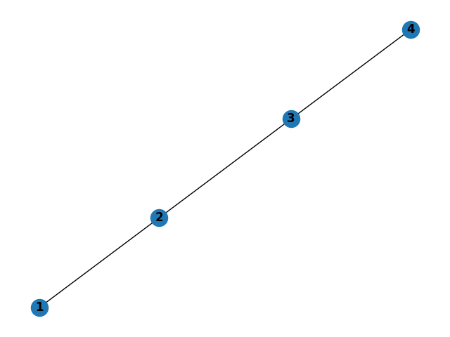
Logic:
- traversal from node 1 should do each in order
- trivial shortest paths
Triangle and Rectangle Tests
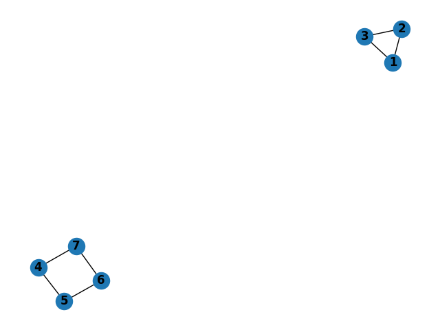
Logic:
- Traversal from node 1 should not include any nodes in the square
- Traversal from node 4 should not include any nodes in the triangle
- There should be no shortest paths between the nodes in the triangle and the nodes in the square.
Unbalanced Kite Tests
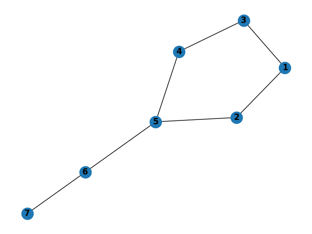
Logic:
- Shortest path from node 1 to node 7 should be through node 2, not node 3
- Traversal from node 1 should be via depth first search (recursion ordering based on order of edges in graph construction)
Referenced Paper
Structuring Depth First Search Algorithms in Haskell
David King and John Launchbury. Proc. ACM Principles of Programming Languages, San
Francisco, 1995.
Appendix
Binary Search Tree Implementation
As demonstrated in the course by Professor Beckman, here is the implementation of a few functions for binary search trees. The elegance and simplicity demonstrates the utility of the Haskell programming language.
data Tree a = Node a (Tree a) (Tree a)
            | Empty
    deriving (Show)

add :: (Ord a) => a -> Tree a -> Tree a
add a Empty = Node a Empty Empty
add a (Node b left right)
    | a <= b = Node b (add a left) right
    | otherwise = Node b left (add a right)

find :: (Ord a) => a -> Tree a -> Bool
find a Empty = False
find a (Node b left right)
    | a == b = True
    | a < b = find a left
    | otherwise = find a right

lookupBST :: (Ord k) => k -> Tree (k,v) -> Maybe v
lookupBST k Empty = Nothing
lookupBST k (Node (a,b) left right)
    | k == a = Just b
    | k < a = lookupBST k left
    | otherwise = lookupBST k right

mergeChildren :: (Ord a) => Tree a -> Tree a -> Tree a
mergeChildren Empty right = right
mergeChildren left Empty = left
mergeChildren left (Node r Empty subright) = Node r left subright
mergeChildren left (Node r subleft subright) = Node r (mergeChildren left subleft) subright

delete :: (Ord a) => a -> Tree a -> Tree a
delete a Empty = Empty
delete a (Node x left right)
    | a > x = Node x left (delete a right)
    | a < x = Node x (delete a left) right
    | otherwise = mergeChildren left right